Quantum Programming with High School Math: Part 1

Recap on Previous Articles

To recap, I previously introduced how to use a Hadamard gate to transform a qubit into a superposition state and how to add a CNOT gate to quantum entangle two qubits. In the latter article, I posed a bonus question at the end of the article, and the answer in QuICScript is

bash

IX,HI,CN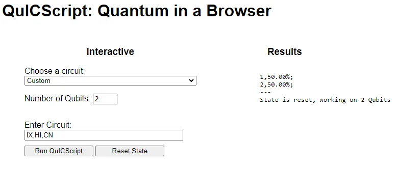

Diagram 1. QuICScript execution results for a Bell state with negatively correlated output states upon measurement.

Motivation

Several friends, after having read my earlier articles on quantum programming, asked if I could share the math behind quantum mechanics (QM) to better appreciate how superposition and quantum entanglement of quantum states work.

I went to read up on the math necessary for quantum programming and found out that a QM pioneer (John von Neumann) observed that all of quantum mechanics can be described by linear algebra. In addition, complex numbers are used to describe the amplitudes and phase difference for the two basis quantum states, namely |0⟩ and |1⟩.

At this juncture, I was pleasantly surprised to discover that my Singapore high school education had already equipped me with the foundations in matrix operations and complex numbers. Lucky me! If I recall correctly, for the past 20+ years, students in Singapore have been taught matrix operations in the 'O' Levels syllabus and complex numbers in the 'A' levels syllabus.

Syllabus Overview of QM Math Series

Initially, I planned on compressing the entire math material into one article. As I continued to add material into the article, I increasingly felt that the layman reader is going to become overwhelmed by the deluge of mathematical content. Even my elementary schooler casually suggested, "Daddy, I think you should break down the material into smaller articles," when he saw my predicament. [chuckle]

With this consideration, in this article, I will limit the scope to how to represent the state of a qubit in two mathematical notations, namely the Bra-ket notation (also known as Dirac notation) and the vector notation. Although complex numbers are used in QM linear algebra, I will also limit to using real numbers in this article.

Once you grasp the mathematical understanding of a qubit, you will be able to determine the probability that a qubit (in superposition state) collapses into one of its basis states upon measurement.

Math Description of a Qubit

Recall that a qubit can be in one of its two basis states, namely |0⟩ and |1⟩, or in a superposition of both basis states. This quantum state of the qubit |Ψ⟩ can be described as a linear combination of two complex numbers α and β, where α describes the amplitude that the qubit is in the |0⟩ state and β describes the amplitude that the qubit is in the |1⟩ state.

Dirac Notation and Vector Notation

We can represent this linear combination in two notations, namely the Dirac notation and the 2x1 vector notation shown below.

|Ψ⟩ = α |0⟩ + β |1⟩ = [\begin{matrix} α \\ β \end{matrix}]

Math for Basis States of a Qubit

To represent qubit |Ψ⟩ in the logical zero state, α is one and β is zero. The notations for a qubit in logical zero state is shown below.

|Ψ⟩ = |0⟩ = [\begin{matrix} 1 \\ 0 \end{matrix}]

Vice versa, to represent a qubit |Ψ⟩ in the logical one state, α is zero and β is one. The notations for a qubit in logical one state is shown below.

|Ψ⟩ = |1⟩ = [\begin{matrix} 0 \\ 1 \end{matrix}]

Math for Superposition State of a Qubit

To represent a qubit |Ψ⟩ in a superposition of its basis states, both α and β have non-zero values. Based on this definition, you may have noticed (intuitively) that there can be an infinite number of superposition states with different α and β values.

One superposition state, that you will frequently encounter in quantum programming, has both α and β equals to one over square root of 2. The notations for a qubit in this superposition state is shown below.

|Ψ⟩ = \frac{1}{\sqrt{2}} |0⟩ + \frac{1}{\sqrt{2}} |1⟩ = \frac{1}{\sqrt{2}} [\begin{matrix} 1 \\ 1 \end{matrix}]

QM Constraint for α and β Values

In the above three examples, the values for α and β may seem to have been arbitrarily chosen without any constraints. However, values for α and β must obey a QM constraint (known as the Born rule) to describe a valid quantum state of a qubit (or in technical terms, a coherent superposition of basis states).

According to the Born rule, you can determine the probabilities of observing each basis state upon measurement of a qubit in superposition. The probability calculation for each basis state is to take the square of the modulus of the associated amplitude (α for |0⟩ and β for |1⟩).

The mathematical constraint of the Born rule is that the total sum of probabilities must equal to 1. The notations for this QM constraint is shown below.

{|α|}^{2} + {|β|}^{2} = 1

Calculating Probability to Measure a Basis State

Let us use the third example, which has a qubit |Ψ⟩ in superposition state with both α and β equals to one over square root of 2. If we measure this qubit |Ψ⟩, the probability to observe |0⟩ or |1⟩ is 50% each. We can verify this as shown below.

{|α|}^{2} = {(\frac{1}{\sqrt{2}})}^{2} = \frac{1}{2}

Review

In this article, we learnt how to represent the quantum state of a qubit in both Dirac notation and vector notation. We also learnt how the mathematical representation can describe each of the two basis states (|0⟩ and |1⟩) and a superposition of the two basis states.

We learnt about the Born rule, which imposes a constraint on values for α and β to describe a valid quantum state of a qubit. Using the mathematical definition of the QM constraint, we are able to determine the probability that a qubit (in superposition state) collapses into one of its basis states upon measurement.

In the next article, I will introduce how to represent some quantum gate operations as matrices and how we can use matrix multiplication to describe quantum state transformations.

Bonus Question

A qubit |Ψ⟩ has been transformed into a superposition state described in the notations below. Upon a measurement of the qubit, what are the probabilities you will observe |0⟩ or |1⟩?

$|Ψ⟩ = \sqrt{\frac{1}{3}} |0⟩ + \sqrt{\frac{2}{3}} |1⟩ = [\begin{matrix} \sqrt{\frac{1}{3}} \\ \sqrt{\frac{2}{3}} \end{matrix}]$

See Answer

Upon measurement of the qubit, we will observe |0⟩ with $\frac{1}{3}$ probability and observe |1⟩ with $\frac{2}{3}$ probability. The math for this is as follow

Probability of |0⟩ $= {|α|}^{2} = {\sqrt{\frac{1}{3}}}^{2} = \frac{1}{3}$

Probability of |1⟩ $= {|β|}^{2} = {\sqrt{\frac{2}{3}}}^{2} = \frac{2}{3}$

Author

Nicholas Ho

Nicholas seriously enjoys learning new knowledge. He is so serious about it that his hobby is to collect hobbies. His most enduring hobby, since 1997, is to continuously explore the ever-evolving domains of applied cryptography, software development, and cybersecurity. His latest aspiration is to add the word quantum in front of each of these 3 domains. Nicholas is currently a Senior Cryptographic Engineer at pQCee.com. Akin to many Singaporeans, he also enjoys collecting popular certifications, including a CS degree, an Infocomm Security masters, CISSP, and CISA.

Search