A Guide to Shor's Algorithm: Part 2 - How to Write a Quantum Fourier Transform Program

Articles in the Series

This article is part of a series. The other articles are:

• A Guide to Shor's Algorithm: Part 1 - How to Break RSA
• (coming soon) A Guide to Shor's Algorithm: Part 3 - How to Write a Quantum Phase Estimation Program

Introduction

Recall in the earlier Part 1 article, Shor's algorithm implements both the exponent factoring method and discrete Fourier transform approach in the quantum phase estimation algorithm. The result is a quantum program that contains a quantum phase estimation (for the function \(U = a^r \mod N\)) coupled with an inverse quantum Fourier transform.

In this article, as a fundamental concept before going onto the full Shor's algorithm, I will show how to develop a quantum program for the quantum Fourier transform (QFT) and how to build a multi-qubit QFT.

What is Fourier Transform?

The Fourier transform is a mathematical function that decomposes an input signal (that varies with time) into component oscillations (e.g., sines & cosines) associated with a range of specified frequencies. In slightly more technical terms, the Fourier transform converts a time-domain signal into a frequency-domain representation (also known as conversion to Fourier basis).

Given the Fourier basis of a signal, the original input signal can be reconstructed by adding together the component oscillations. This reversal process is also known as the inverse Fourier transform.

The Fourier transform can only be applied on a continuous signal. As such, it is primarily used in the theoretical analysis of signals in the domains of physics and engineering.

Discrete Fourier Transform

In order to digitalize the "analog" Fourier transform, an effective solution was to model discrete values as a wave and apply the Fourier transform. The resulting function is known as the discrete Fourier transform (DFT).

The fast Fourier transform (FFT) is a further optimized implementation (e.g., higher efficiency and less memory requirements) of DFT for computers. As a result, FFT (instead of standard DFT) is widely implemented in digital signal processing, including applications like MP3 audio compression, image processing, and communication systems like Wi-Fi.

How DFT works, in a nutshell, is to first digitize a continuous signal (by sampling at regular time intervals) into a sequence of \(N\) discrete amplitude values \(x_0, x_1, \ldots , x_{N-1}\). In conformance to digital representation of data, the number of signal samples taken is usually a power of 2, resulting \(N = 2^n\) samples. 

DFT then applies a Fourier transform on this sequence to generate a frequency-domain representation (aka Fourier basis) \(y_k\) for wavenumber values \(k = 0, 1, \ldots , {N-1} \). (In technical terms, the wavenumber \(k\) is the number of complete waves that fit into interval \([-\pi,\pi]\). As such, some people like to informally refer to \(k\) as the fundamental frequency in Fourier basis.) The DFT to calculate each \(y_k\) value is defined as

$$y_k = DFT(k) = \displaystyle\sum_{j=0}^{N-1} e^{\frac{-2\pi ikj}{N}} \sdot x_j$$

In the equation above, note that the phase information for each component of the signal is encoded in the complex number component of \(y_k\). Also, similar to Fourier transform, the reverse process can be performed by the inverse DFT.

Quantum Fourier Transform

The quantum Fourier transform (QFT) is analogous to the quantum version of the DFT. However, QFT handles conversion across two quantum states (from quantum state in computation basis to quantum state in Fourier basis), instead of the time and frequency domains mentioned earlier.

In addition, QFT applies the transformation on all sequence values simultaneously instead of iteratively operating on them. In order to achieve this, the input sequence and output values needs to be encoded as a quantum state in a qudit (aka multi-state quantum computation unit).

The input sequence of N discrete amplitude values \(x_0, x_1, \ldots , x_{N-1}\) is encoded as a quantum state in a qudit \(\ket{x}\). This quantum representation of the input values is known as the computation basis. The following shows the encoding of the sequence as a quantum state:

$$ \ket{x} = \begin{pmatrix} x_0 \\ x_1 \\ x_2 \\ \cdots \\ x_{N-1} \end{pmatrix} $$

The QFT output sequence \(y_0, y_1, \ldots , y_{N-1}\) is encoded as a quantum state in a qudit \(\ket{y}\). Each \(y_k\) represents a component basis quantum state from the decomposition of the input quantum state. This quantum representation of output values is known as the Fourier basis. The following shows the QFT output as another quantum state:

$$ \ket{y} = \begin{pmatrix} y_0 \\ y_1 \\ y_2 \\ \cdots \\ y_{N-1} \end{pmatrix} $$

The definition of QFT has some variations from DFT. One of it is the inclusion of a normalization parameter \( \frac{1}{\sqrt{N}} \) to conform to the quantum mechanical constraint of the Born rule. The \(n\)-state qudit QFT (in Dirac notation) is defined as

$$ QFT \ket{x} = \frac{1}{\sqrt{N}} \displaystyle\sum_{j=0}^{N-1} e^{\frac{2\pi ixj}{N}} \ket{j} = \ket{y} , N = 2^n $$

If we express the above equation in the form of qubits, we can first convert \(j\) into binary form \( \ket{j} = \ket{j_1 j_2 \ldots j_n} \). In this binary form, \(j_1\) is the most significant qubit and \(j_n\) is the least significant qubit. The \(n\)-qubit QFT can be re-written as the following form

$$ QFT \ket{x} = \frac{1}{\sqrt{N}} \displaystyle\sum_{j=0}^{N-1} e^{2\pi i x \textstyle\sum_{p=1}^{n} \frac{j_p}{2^p}} \ket{j_1 j_2 \ldots j_n} = \ket{y} $$

In the qubit form above, one interesting observation is that the QFT has converted integer binary input in computational basis to fractional binary output in Fourier basis. For further mathematical clarity, for an integer in binary representation \(j=j_1 j_2 \ldots j_n\), it can be rewritten as a fractional binary representation \( \frac{j}{2^n} = \textstyle\sum_{p=1}^{n} \frac{j_p}{2^p}\). This is also the reason why precision for \(\ket{y}\) increases when the number of qubits \(n\) increases.

Let us take the summation term out of the power, as shown below, to facilitate subsequent term expansion.

$$ QFT \ket{x} = \frac{1}{\sqrt{N}} \displaystyle\sum_{j=0}^{N-1} \displaystyle\prod_{p=1}^{n} e^{\frac{2\pi i x j_p}{2^p}} \ket{j_1 j_2 \ldots j_n} = \ket{y} $$

When we expand the product term, we can see that each qubit is neatly associated with a corresponding complex number term as follows

$$ QFT \ket{x} = \frac{1}{\sqrt{N}} (\ket{0} + e^{\frac{2\pi i x}{2^1}} \ket{1}) \otimes (\ket{0} + e^{\frac{2\pi i k}{2^2}} \ket{1}) \otimes \ldots \otimes (\ket{0} + e^{\frac{2\pi i k}{2^n}} \ket{1}) = \ket{y} $$

In the equation above, the interesting observation is that QFT encodes the phase information for each component of the signal in the phase rotation of each qubit output. With the \(n\)-qubit QFT expressed in this form, we can now intuitively convert the equation into quantum circuits.

Programming Circuits for Quantum Fourier Transform

In the expanded form of \(n\)-qubit QFT shown above, the term \(e^{\frac{2\pi i k}{2^n}}\) can be converted into equivalent phase rotation gates with phase rotation \(\frac{\pi}{2^n}\).

1-qubit QFT

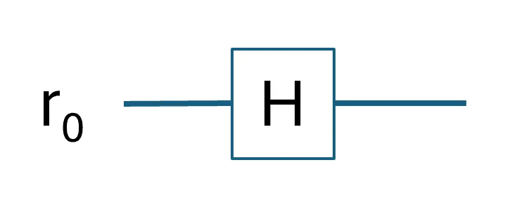
If we wish to build a 1-qubit QFT, we will need to implement a quantum gate that performs a \(\frac{\pi}{2}\) phase rotation (corresponding to the term \((\ket{0} + e^{\frac{2\pi i k}{2^1}} \ket{1})\)) when \(\ket{r_0} = \ket{1}\). Based on the mathematics, the Hadamard (H) gate fulfils this operation. As such, the 1-qubit QFT involves only one H gate (as shown in Diagram 1 above).

2-qubit QFT

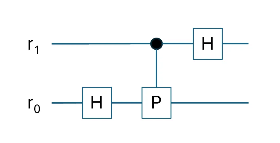
To extend the circuit to a 2-qubit QFT for \(\ket{r} = \ket{r_1 r_0}\), we will need to implement a combination of two different phase rotations on entangled qubits \(\ket{r}\). Specifically, apply a \(\frac{\pi}{2}\) phase rotation on \(\ket{r}\) whenever \(\ket{r_1} = \ket{1}\), and apply a \(\frac{\pi}{4}\) phase rotation on \(\ket{r}\) whenever \(\ket{r_0} = \ket{1}\).

This linear combination of phase rotations corresponds to the terms \((\ket{0} + e^{\frac{2\pi i k}{2^1}} \ket{1}) + (\ket{0} + e^{\frac{2\pi i k}{2^2}} \ket{1})\), and is realized as the circuit shown in Diagram 2 above.

3-qubit QFT

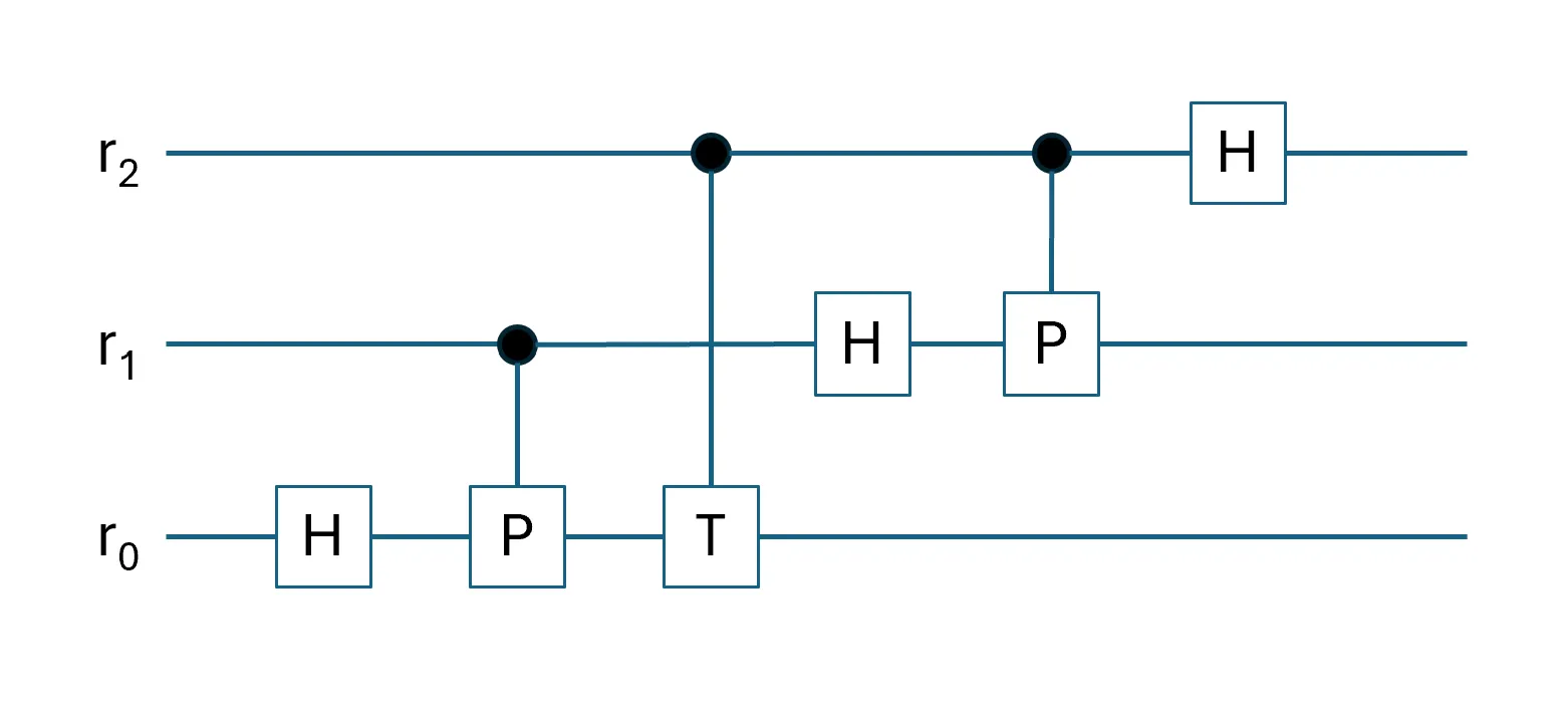
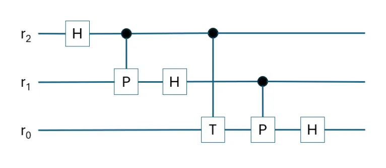
In the same approach to increasing the QFT size, to extend the circuit to a 3-qubit QFT for \(\ket{r} = \ket{r_2 r_1 r_0}\), we will need to implement a combination of three different phase rotations on entangled qubits \(\ket{r}\). Specifically, apply a \(\frac{\pi}{2}\) phase rotation on \(\ket{r}\) whenever \(\ket{r_2} = \ket{1}\); apply a \(\frac{\pi}{4}\) phase rotation on \(\ket{r}\) whenever \(\ket{r_1} = \ket{1}\); apply a \(\frac{\pi}{8}\) phase rotation on \(\ket{r}\) whenever \(\ket{r_0} = \ket{1}\). This linear combination of phase rotations is realized in the circuit shown in Diagram 3 above.

To extend to n-qubit QFT circuits for \(n > 3\), you can follow the same approach to implement a combination of \(n\) different phase rotations on entangled qubits \(\ket{r}\).

Inverse QFT

The quantum circuit for the inverse QFT is surprisingly easy to derive from a graphical point of view. All you need to do is to reflect the sequence of the quantum gates laterally. One example is to perform a lateral reflection of the 3-qubit QFT (in Diagram 3 above) to get the 3-qubit inverse QFT (in Diagram 4 above).

$$ QFT^{\dagger} \ket{y} = \frac{1}{\sqrt{N}} \displaystyle\sum_{j=0}^{N-1} e^{-\frac{2\pi iyj}{N}} \ket{j} = \ket{x} , N = 2^n $$

For those interested in the mathematical definition for inverse QFT (as shown above), inverse QFT has a different exponent sign as compared to the QFT.

Conclusion

In this article, we learnt how to create n-qubit QFT and inverse QFT quantum circuits for any arbitrary \(n >=1\) using common quantum gates. We also learnt that QFT converts an integer binary input into a fractional binary output, which is why precision for QFT output increases with a larger n-qubit QFT.

At this point, if you are thinking that the QFT is the only quantum circuit to produce a quantum output in Fourier basis, then you are mistaken. In addition to the QFT, the quantum phase estimation (QPE) circuit is another approach to produce a quantum output in Fourier basis, and Shor's algorithm uses a combination of QPE and inverse QFT to achieve factorisation.

In the next part of this series, I will go into how to create the quantum phase estimation circuit for Shor's algorithm.