
A Guide to Shor's Algorithm: Part 1 - How to Break RSA
Articles in the Series
This article is part of a series. The other articles are:
Introduction
RSA encryption, a cornerstone of modern digital security, relies on the difficulty to factor a large composite number made up of two prime numbers. In case you were wondering, large here means a number consisting of at least one hundred digits.
The most efficient classical algorithm to factorize a composite number is the General Number Field Sieve (GNFS) with a general time complexity of \(O(e^{\sqrt[3]{(\ln n) (\ln \ln n)^2}})\). The quantum equivalent of a factorization algorithm is known as Shor's algorithm, which can factorize a composite number with a reduced general time complexity of \(O((\ln n)^3)\). Computer science academia frequently refers to this reduction as an improvement from exponential time to polynomial time.
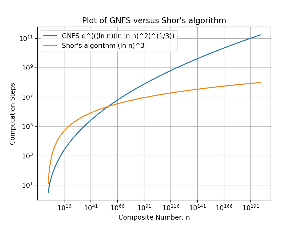
To help layman readers better appreciate the impact of the performance speed up, in Diagram 1 above, as the composite number (n) to be factored increases beyond around 60 digits, the time taken by Shor's algorithm scales much better than GNFS. As a result, since RSA-2048 utilizes a composite number with around 620 digits, Shor's algorithm makes factorization more feasible than GNFS.
This giant leap of improvement to factor a large number is the key reason that Shor's algorithm shot to fame worldwide. If you ask anyone which quantum algorithm first comes to mind, it is without a doubt, Shor's algorithm.
Overview of Shor's Algorithm
The brilliance behind Shor's algorithm is that it integrates techniques across multiple domains to enable quantum factorization.
In the mathematics domain, among the various factorization techniques, Peter Shor selected the exponent factoring method that involves a finding hidden period of a composite number (e.g., N = 3x7 = 21) to factor the composite number.
In the physics and engineering domains, he adopted the discrete Fourier transform (DFT) approach to determine the hidden period of a composite number in the exponent factoring method.
Finally, in the quantum computing domain, he used the quantum phase estimation algorithm to integrate the exponent factoring method and DFT approach together, resulting in Shor's algorithm.
In the following sections, I will guide you on how to perform Shor's algorithm.
Quantum Factorization of 21
Before I go into the actual algorithm, I will first highlight the key parts of the factoring method, so that you will have a better context on why we are doing certain steps and what we are looking for.
Exponent Factoring Method
In the exponent factoring method, we choose a random number \(a\) for a target composite number \(N\), such that the equation \(a^r \mod N\) will result in a repeating sequence when we iteratively substitute \(r = 1\ldots N\) into the modulus equation.
We will then attempt to find the smallest value of \(r\) associated with the first occurrence of \(a^r \mod N=1\), which is the hidden period of the repeating sequence (or also known as the order of the sequence). Knowing the hidden period \(r\) will provide a high chance to determine the factors of \(N\).
One of the two factors of \(N\) can be subsequently derived by calculating the greatest common divisor (GCD) of \(a^{\frac{r}{2}} \pm 1\) with \(N\). Once a factor \(g\) has been found, the other factor can be easily derived by calculating \(\frac{N}{g}\).
In view of the above, the following conditions must be satisfied for the method to work:
- The random number \(a\) must be co-prime to \(N\). In other words, other than \(1\), the numbers \(a\) and \(N\) do not have common factors.
- The hidden period \(r\) must be an even number. Otherwise, the factoring attempt must be restarted with a different \(a\) value.
Algorithm Steps to Factor 21
Having shared the approach and constraints of the exponent factoring method, let us dive into the steps needed to perform quantum factorization on the target \(N=21\).
Step 1: Select a random a
Let us choose \(a=2\), as 2 is co-prime to 21. This step is done on a digital computer (aka classical computer).
Overview of next step, find the hidden period r
There are two methods to find the period \(r\). One is the classical method (labelled Option #1), and the other is the quantum method (labelled Option #2). I included both methods to facilitate understanding for readers seeing Shor's algorithm for the first time.
(Option #1) Step 2: Brute force to find period r
This step is executed on a classical computer. We will iteratively test every value of \(r\), in increasing order, for the modulus function and locate the first occurrence of \(2^r \mod 21 = 1\). Run the code below to perform a brute force on all possible values of \(r\) to find the hidden period.
python
for r in range(1, 22):
    print(pow(2, r, 21))
We will observe a sequence repeating after every 6 elements (similar to the sequence shown in the table below).
| \(r\) | 1 | 2 | 3 | 4 | 5 | 6 | 7 | 8 | 9 | 10 | 11 | 12 | ... |
| \(2^r \mod 21\) | 2 | 4 | 8 | 16 | 11 | 1 | 2 | 4 | 8 | 16 | 11 | 1 | ... |
In this repeating sequence, the first occurrence of \(2^r \mod 21 = 1\) occurs at \(r=6\). Thus, we found the hidden period to be \(r=6\).
(Option #2) Step 2a: Run Shor's algorithm targeting N=21
This step is executed on a quantum computer. Set up and execute Shor's algorithm to generate an intermediate output, which contains hints with a high chance to reveal the hidden period \(r\).
In place of a quantum computer, we can execute a quantum program (written in QuICScript) via the Quantum-in-a-Browser quantum emulator.
First, open Quantum-in-a-Browser in a new tab, download and save the 12-qubit quantum program for "shors21". Next, on the left side of the Quantum-in-a-Browser interface, click the "Choose File" button to upload and execute the quantum program.
You will see an output containing states spanning from 0 to 127 on the right side of the Quantum-in-a-Browser interface. These states also have probabilities paired with each line entry of the state.
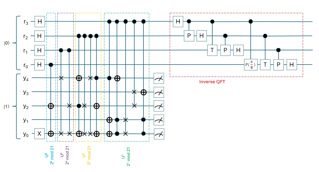
To give you a feel of how a quantum program for Shor's algorithm targeting \(N=21\) will look like, see Diagram 2 above. For avoidance of benefit of doubt, the 12-qubit quantum program we used in QuICScript earlier implements 7 qubits for \(r\) (instead of 4 qubits) in order to achieve higher precision to determine the hidden period.
(Option #2) Step 2b: Use continued fractions to find hidden period r
This step is executed on a classical computer. We will now analyze the output from Step 2a earlier and look out for output states with significantly higher probabilities (or peak values). Let us choose peak values with probabilities more than 10%. You will notice that peak values satisfying our criteria occur at output states 0, 42, 53, 85 and 106.
Note
We have the luxury to select output states with higher probabilities because we are using output from a quantum emulator. With a quantum computer, you can only measure one random output state per run of Shor's algorithm. As such, you will likely need to repeat Shor's algorithm multiple times to increase the chances of measuring a peak value that reveals the hidden period \(r\).Next, we will need to use an iterative mathematical process called continued fractions on each of the peak values to reveal the hidden period \(r\). We can ignore processing the peak value at 0 as this is a peak value that appears in all runs of Shor's algorithm regardless of parameters.
As it can get quite tedious to calculate continued fractions for each peak value by hand, I automated the process to select candidate values for \(r\) with the script below. Run the script below on peak values 42, 53, 85 and 106.
python
from fractions import Fraction

def get_likely_period(peak_value, no_of_qubits_for_r, a, n):
    r_candidates = set()
    # Generate denominators of all continued fractions for peak_value
    for d in range(2, n):
        frac = Fraction(peak_value, 2**no_of_qubits_for_r).limit_denominator(d)
        # Accept condition for r candidates: denominator >= 2 and even number
        if frac.denominator > 1:
            if frac.denominator % 2 == 0:
                r_candidates.add(frac.denominator)
    # Filter only candidates that result in a ^ r mod n = 1
    valid_r = set()
    if not r_candidates:
        return valid_r
    for r in sorted(r_candidates):
        if pow(a, r, n) == 1:
            valid_r.add(r)
    return valid_r

# Change the first argument to check a different peak value
print(get_likely_period(42,7,2,21))
Having checked the four peak values, you will observe that peak values 53 and 106 yield candidate values \(r=6,12\). Recall that the hidden period is the first occurrence where \(2^r \mod 21=1\), thus we select the smallest candidate value \(r=6\) as the answer from Shor's algorithm.
Step 3: Use \(\frac{r}{2}\) to find the factors of 21
This step is executed on a classical computer. We let \(x = 2^{\frac{6}{2}} = 2^3 = 8\) and find the GCD of \(x\pm1\) with \(21\) to derive the factors of 21. Run the code below to derive the factors of 21.
python
import math
print(math.gcd(7,21))
print(math.gcd(9,21))
You will observe that both GCDs, coincidentally, return the factors 7 and 3 respectively.
How Factorization Breaks RSA
In the earlier section, you derived the factors of 21 using Shor's algorithm. I will now share how factorization of a composite number can break RSA.
Case Study
Let us assume that I published my RSA public key with the following parameters, \(N=pq=21, e=11\), where \(p\) and \(q\) are prime factors of \(N\). I encrypt a message \(M=12\) with RSA encryption algorithm \(C = M^e \mod N\), where \(C\) is the ciphertext.
$$C = 12^{11} \equiv 3 \pmod {21}$$
As an attacker, you applied Shor's algorithm on my public key and derived the factors \(p=3\) and \(q=7\). With the factors revealed, you can now derive my private key \(d\) with the following RSA private key derivation algorithm \(d = e^{-1} \mod {(p - 1)(q - 1)}\)
$$d = 11^{-1} \equiv 11 \pmod {12}$$
Note
In this case study, it just so happens that both private and public keys have the same value. With a properly chosen set of RSA parameters, the private key is always different from the public key.With my private key \(d=11\), you can now decrypt my ciphertext \(C\) to get my original message \(M\) using the RSA decryption algorithm \(M = C^d \mod N\)
$$M = 3^{11} \equiv 12 \pmod {21}$$
Having gone through the case study, we can now see that once you factorize the composite \(N\) parameter of the RSA public key, the security assurance by the RSA algorithm is no longer guaranteed.
Conclusion
In this article, we learnt that Shor's algorithm enables feasible factorization of large composite integers with \(\gg 60\) digits, which was previously deemed impractical with GNFS . We also had a step-by-step walkthrough on how to apply Shor's algorithm to factorize the composite integer 21, and subsequently used the factors to break RSA.
In the next part of this series, I will go into deeper technical detail on how to design the quantum program for Shor's algorithm using only common quantum gates.
Author
Nicholas Ho
Nicholas seriously enjoys learning new knowledge. He is so serious about it that his hobby is to collect hobbies. His most enduring hobby, since 1997, is to continuously explore the ever-evolving domains of applied cryptography, software development, and cybersecurity. His latest aspiration is to add the word quantum in front of each of these 3 domains. Nicholas is currently a Senior Cryptographic Engineer at pQCee.com. Akin to many Singaporeans, he also enjoys collecting popular certifications, including a CS degree, an Infocomm Security masters, CISSP, and CISA.