A Guide to STARK Part I: The General Idea

Zero-Knowledge Scalable Transparent Argument of Knowledge (zk-STARK or just STARK) is a zero-knowledge proof system that is centered around polynomials. 

STARK relies on the mathematical concept that changing a single point on a polynomial creates a new polynomial drastically different from the original.

The concept is a stark (sorry) contrast to the multi-party computation in-the-head (MPCitH) paradigm, which relies on the concept of allowing \(n\) parties to secret-share an input, do their computations in private, revealing some of these the computations to check that the computations are not bogus.

This series will be focused on understanding STARK with frequent use of mathematical concepts, but this post discusses the general idea behind STARK. 

Polynomials: The STARK Core

Let's start by explaining the mathematical concept that is the foundation of STARK: polynomials.

A function \(f(x)\) is called a (single-variable) polynomial if it can be expressed in this form:

$$A(x) = a_0 + a_1x + a_2x^2 + a_3x^3 + \dots + a_nx^n$$

where \(A(x)\) is called a polynomial of degree \(n\) if \(a_n \ne 0\).

Given \(n+1\) data points on a graph, the points can be interpolated into a polynomial \(A(x)\) of degree at most \(n\), and this polynomial is unique. One way to interpolate the points is to use Lagrange polynomial interpolation.

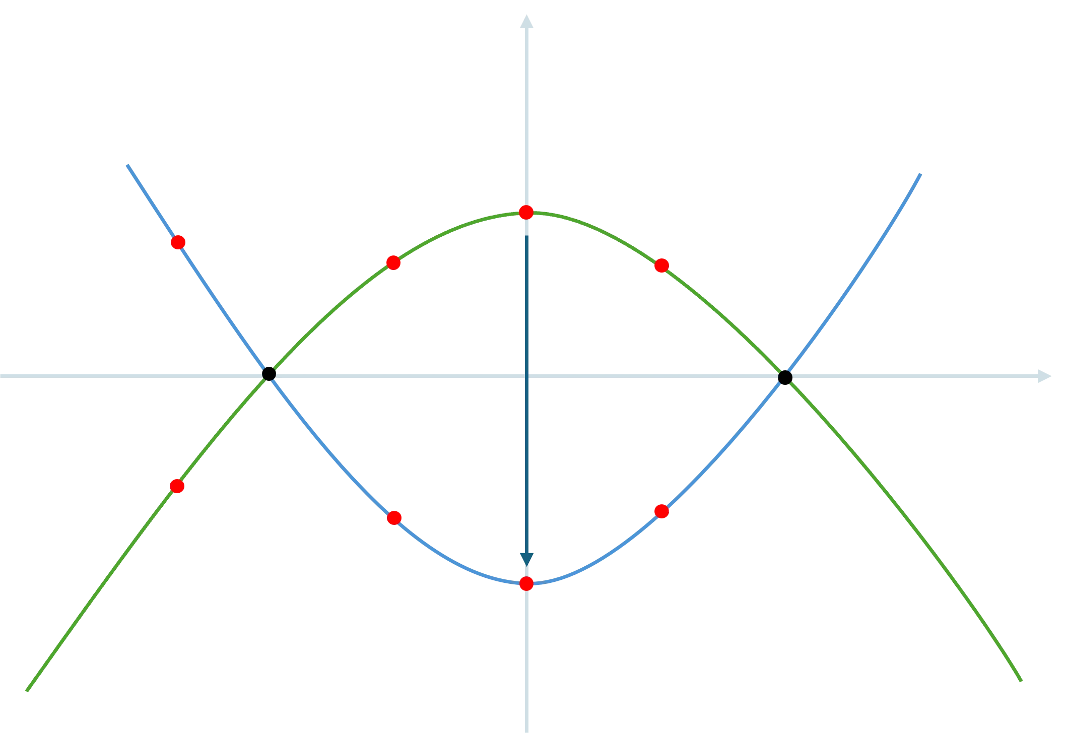
For example, given three data points \((-1, 0), (0, 1), (1, 0)\), there is only one way to draw a polynomial of degree at most 2 through them: \(A(x) = -x^2 + 1\). The green curve in the graph below represents this polynomial \(A(x)\).

Since \(n+1\) points must interpolate into a unique polynomial of degree at most \(n\),

• Any deviation in the data points result in a different interpolated polynomial \(B(x)\), also at most degree \(n\), and

• \(A(x)\) and \(B(x)\) have at most \(n\) common points. If they had \(n+1\) or more common points, they would have interpolated into the same polynomial.

For example, if we moved the data point \((0, 1)\) to \((0, -1)\), the new polynomial becomes \(B(x) = x^2 - 1\). The blue curve below represents this polynomial \(B(x)\). Notice that the points between the two polynomials are different at every point except -1 and 1.

Now, suppose we have a polynomial \(P(x)\) of degree 1,000. We pick and note down 2,000 points on this polynomial.

If we have a different polynomial \(Q(x)\) also of degree 1,000, then \(P(x)\) and \(Q(x)\) can have at most 1,000 points in common.

That means, all the other points must be different in \(Q(x)\); so \(P(x)\) and \(Q(x)\) must have at least 1,000 different points.

We can extend this behaviour as much as we want. If we have noted 10,000 (instead of 2,000) points from \(P(x)\), at least 9,000 points would have been different. If we have noted 100,000 points, at least 99,000 points would have been different.

Tying back to ZKPs

To recap, a zero-knowledge proof is a proof that a prover creates to convince a verifier that the prover knows a secret, without revealing the secret itself.

STARK is a zero-knowledge proof system used to prove computational integrity of a secret - that a party reports the actual computation done on a secret, instead of a result more favourable to the party.

The polynomial \(P(x)\) above loosely represents such a genuine proof. During the process of the computation, the result of each step of the computation is translated into data points. The points are then interpolated into a polynomial, such that it satisfies, for example \(P(x) = 0\) for all \(x\) at the data points.

The polynomial \(Q(x)\) represents a fake proof that a malicious prover could create to attempt to cheat the verifier. Without knowing the actual secret that derived \(P(x)\), perhaps the best the malicious prover could come out with is a \(Q(x)\) such that \(Q(x)=0\) is true for only some of the points.

To check the proof, a verifier samples points on the prover's polynomial.

Drawing from the previous example, an honest prover derives, from his secret, a polynomial \(P(x)\) of degree 1,000 that fits the constraint \(P(x)=0\), and notes down 2,000 points.

A malicious prover creates a \(Q(x)\) of the same degree, also noting down 2,000 points.

A verifier that samples the points randomly. However, since at least 1,000 out of 2,000 points from \(Q(x)\) are different from \(P(x)\), the probability of the malicious prover getting caught is at least 50%.

Notice that we can boost this probability if we noted down even more points.

• If 10,000 points have been noted down, the probability of getting caught goes up to 90%.

• If 100,000 points have been noted down, the probability of getting caught goes up to 99%.

We can even further boost it when the verifier samples multiple times.

• If the verifier samples 16 times, the probability would become \(1-10^{-32}\). This effectively makes the difficulty for the malicious prover to avoid getting caught as good as finding a hash collision!

What is done here is essentially an error-boosting algorithm - a single point of error results in an easily measurable difference.

Other Components

While the concept covered in this post is very simple and basic, it is only a naive view of the real concepts and clever engineering tricks that STARK depends on.

A few of these will be covered in this STARK series, including:

• translating a real problem into a polynomial through constraints,

• checking data points follow a low-degree polynomial, a.k.a., low-degree testing, so that a malicious prover cannot invent data points outside of a polynomial to satisfy the constraints, and

• designing a sound and efficient sampling method so that the number of checks by verifier can be significantly fewer than the number of data points, hence reducing proof size.